mlwkdb by ro

q principal component analysis

Posted in kdb+, q, statistics by machine learning w kdb on October 23, 2009

PCA is a pattern recognition algorithm that highlights similarities and differences in a dataset. It can also be used to optimally (least information loss) reduce the dimension (given by the number of variates) of a dataset by projecting the data (in the least squares sense) onto a few of its principal (high variability) components (dimensions in transformed space). A reduction to 2 components (best approximating plane) can be used to capture and visualize the majority of the variance in the dataset.

The components correspond to the new transformed basis and don’t necessarily have a one-to-one correspondence with the original variates; there are two ways to think about why we would consider dropping components in the transformed space:

  1. if certain variates are redundant (express almost the same information i.e. are highly correlated) then it makes sense to include only a single component to record the information contained in the variates
  2. by rotating and stretching the data into a new basis we are left with components along which there is very little variance; intuitively these components correspond to noise since they fail to record any essential information

Since we are comparing the spreads of variates it makes sense to standardize the data to have zero mean and unit standard deviation.

Given a dataset X_{m \times n} = \{ \vec{x}_1 | \vec{x}_2 | \cdots | \vec{x}_n\} = \{\vec{f}_1, \vec{f}_2, \cdots , \vec{f}_m\} where the n columns are sample vectors and the m rows are feature vectors, we are interested in finding directions in \mathbb{R}^m (the row space) that capture maximal variance. We calculate the center of mass \nu_{m \times 1} = argmin_{\vec{x}} \sum \|\vec{x}_i-\vec{x}\|^2 = \frac{1}{n} \sum_{i=1}^n \vec{x}_i which gives us the mean of each row. The center of mass will serve as the origin of the new basis.

Next we calculate the scatter matrix as the product of the demeaned dataset (subtract the mean of each row from the row so that all the rows have mean zero) with a transposed version of itself: S_{m \times m}=\sum_{i=1}^m (\vec{f}_i - \nu_i)(\vec{f}_i-\nu_i)^T or in matrix form S_{m \times m} = XC_nX^T where C_n is the centering matrix. The entries of the scatter matrix measure the variance of the data in different directions relative to the center of mass; specifically the i-j th entry is the covariance between the ith and jth feature.

Since we are rotating our data into a new basis, what we will need is a measure of the variance of the data set projected onto each axis (infact any arbitrary axis since we need the one with highest variance). To illustrate how we can build such a measure (using only the scatter matrix and any arbitrary unit vector direction) let us project the data onto a line L=\nu+ae representing an axis in the direction e such that \|e \| =1

principal component analysis

The distance of the projected point \vec{f'}_i from the center of mass \nu is then \| \vec{f'}_i - \nu \| = \langle e, \vec{f}_i - \nu \rangle \| e \| = e^T (\vec{f}_i - \nu)

So the total variance or the squared sum of the distances of all the projected points from the center of mass is given by:
var(e) = \frac{1}{m} \sum \| \vec{f'}_i - \nu \|^2 = \frac{1}{m} \sum (e^T (\vec{f}_i - \nu))^2
which after some matrix algebra works out to var(e) = \frac{1}{m} e^T S e.

So now we can calculate the variance of the data projected onto some arbitrary direction e; the principal component is precisely the direction that maximizes this variance: \max_e e^TSe subject to e^Te=1. The lagrangian of this optimization is given by e^TSe - \lambda(e^Te-1) where the \lambda is a slack variable or lagrange multiplier. We apply the lagrangian saddle point equivalence theorem and differentiate with respect to the primal variables 2Se-2 \lambda e = 0 or Se=\lambda e which is in fact part of the eigen-decomposition of the scatter matrix. So the direction along which the projected data has maximized variance is an eigen-vector; but which one? The variance of an eigen-vector is given by var(e) = e^T S e = e^T \lambda e e^T e = \lambda and since we are maximizing the variance \max_e var(e) = \max_e \lambda the eigen-vector with a corresponding maximal eigen-value \lambda is the principal component.

Note if the eigen-values are nearly the same then there is no preferable “principal” component. Also pca is optimal only in the least-squares sense.

Connection to SVD

The svd of the scatter matrix is S=U\Sigma V^T and since the scatter matrix is symmetric S=S^T, we have S=U\Sigma V^T=S^T=V\Sigma U^T which is satisfied only when U=V so we have S=U\Sigma U^T which is exactly the eigen-decomposition so that for S the eigen-values are the singular values. Look here for the general relationship between the eigendecomposition and the svd when the matrix is not square.

Outline of PCA algorithm

  1. Calculate the scatter matrix S
  2. Calculate the SVD of S=U\Sigma U^T
  3. Rearrange the singular values and singular vectors: \tilde{\Sigma} and \tilde{U}
  4. Select a new basis as a subset of the singular vectors \tilde{U}_{1:r}
  5. Project the data onto the new basis X_r = \tilde{U}_{1:r} \cdot X
.qml.mpca:{[x;r] \x is samples (rows) by variates (cols)
 t:-[;avg x] each x;
 t: t $ flip t;
 s:.qml.msvd[t];
 u:s[0][;1+til r];
 :flip[u] $ x;
 };

m:10;
n:800;
x:(m;n)#(m*n)?1f;
.qml.mpca[x;2]

Kernel PCA

Is an extension of PCA for non-linear distributions. We would like to apply PCA in a higher dimensional space \vec{x} \to \phi(\vec{x}); the application of this map to the data set is unnecessary because of the kernel trick. We simply form the kernel matrix and solve this dual problem by finding its singular value decomposition; K \alpha = \lambda \alpha. A feature f_K in the higher dimensional feature space is given by f_K = \sum \alpha_i k(\vec{z}, \vec{f}_i) where \vec{z} is a feature in the original feature space. For a derivation of this result look here or here

Variance Connection, Karhunen Connection

A typical data matrix contains signals each of which has some underlying noise; a reduced rank SVD approximation of the data matrix captures a highest variance mixture of the original signals in a lower dimensional space. The noise is usually associated with the smallest singular values (outliers generally have the least to say about the true distribution of the data because well it is noise and doesn’t belong in the dataset; they have the smallest semi-axis in the transformed unit sphere i.e. they are what the fuck can i explain this better?) which are dropped to form the approximation.

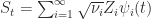
the karhunen–loève representation of a stochastic process

Posted in statistics by machine learning w kdb on October 17, 2009

Consider a continuous time, continuous state space stochastic process \{ S_t : t \in \mathcal{I} \} that has a continuous and compact index set \mathcal{I} and where the random variables S_t are measurable functions from a probability space to a (continuous, measurable) state space:

S_t : (\mathcal{X}, \Sigma_\mathcal{X}, \mu) \to (\mathcal{Y}, \Sigma_\mathcal{Y})

Assume the stochastic process is centered (each random variable is centered) so that \mathbb{E}(S_t)=\int_\mathcal{X} S_t d\mu = 0 then the autocovariance (the variance of the process or signal against a time shifted version of itself) is given by Cov(S_t,S_s) = \mathbb{E}(S_t \cdot S_s) - \mathbb{E}(S_t) \cdot \mathbb{E}(S_s) which given our assumption can be viewed as a kernel

K_{SS}(t,s) = \mathbb{E}(S_t \cdot S_s) = Cov(S_t,S_s)

Let us assume that this kernel is positive, symmetric and square integrable K_{SS}(t,s) \in L^2(\mathcal{X} \times \mathcal{X}) then the resulting integral operator

T_K f(\cdot) : L^2(\mathcal{X}) \to L^2(\mathcal{X}) = \int_{\mathcal{I}} K_{SS}(\cdot,s) f(t) ds

is positive, self-adjoint and compact. It therefore follows from the Spectral Decomposition Theorem that T_K must have a countable set of non-negative eigenvalues \{ \nu_1, \nu_2, \cdots \}; furthermore, the corresponding eigenfunctions \{ \psi_1, \psi_2, \cdots \} must form an orthonormal basis for L^2(\mathcal{X}):

T\psi_i(t) = \int_\mathcal{I} K_{SS}(t,s) \psi_i(s) ds = \nu_i\psi_i(t)

The integral transformation T_K essentially changes the representation of the input function f to an output function (T_Kf) defined in a space that has a basis given by the set of eigenfunctions.

Let us make a stronger assumption (than being square integrable) that the covariance (kernel) function is continuous Cov(S_t, S_s) \in C^0(\mathcal{X} \times \mathcal{X}) then by Mercer’s theorem (page 34) we have that:

Cov(S_t, S_s) = \sum_{i=1}^\infty \nu_i \psi_i(s) \psi_i(t)

where convergence is absolute and uniform in both variables. We define a new set of random variables \{ Z_n, n \geq 0\} based on our original stochastic process:

Z_n = \frac{1}{\sqrt{\nu_n}} \int_{\mathcal{I}} S_t \psi_n(t) dt

that are orthogonal and centered E(Z_n)=0. We can then represent our original stochastic process as an infinite linear combination of orthogonal functions:

S_t = \sum_{i=1}^\infty \sqrt{\nu_i} Z_i \psi_i(t)

where convergence is uniform over the index set \mathcal{I}. It is interesting to note that the orthogonal basis functions used in this expansion are determined by the autocovariance function.

References:
1. Karhunen-Loeve Expansion of Vector Random Processes
2. Large Scale Learning: Dimensionality Reduction

singular value decomposition

Posted in kdb+, statistics by machine learning w kdb on October 7, 2009

The singular value decomposition of a n \times m matrix M is given by

M = U_{(n \times n)} \Sigma_{(n \times m)} {V^T}_{(m \times m)}

where the rows or right-singular vectors of V^T (and the columns or left-singular vectors of U) form a set of orthonormal basis vector directions:

U^T U = I and V^T V=I

The singular value matrix \Sigma is diagonal with entries equal to the square roots of the eigenvalues of the matrix M^TM. If the diagonal entries \sigma_i are sorted in decreasing order then \Sigma is uniquely determined. The same is not true of the left and right singular vectors.

As a geometric transform

Any real matrix maybe viewed as a geometric transformation

M:\mathbb{R}^m \to \mathbb{R}^n : U \Sigma V^T=(hanger)(stretcher)(aligner)

that when applied to a set of data points M \vec{d}_i = U \Sigma V^T \vec{d}_i rotates them in the direction of the right singular vectors \{\vec{v}_1, \vec{v}_2, \cdots , \vec{v}_n \} first and then stretches them in the direction of each of the left singular vectors \{\vec{u}_1, \vec{u}_2, \cdots , \vec{u}_m \} by a factor equal to its corresponding singular values \{\sigma_1, \sigma_2, \cdots , \sigma_n \}. The order of the rotate and stretch is important as it determines the final output space. Note that from M\vec{v}_i = \sigma_i \vec{u}_i, \forall i \leq min(n,m) and M\vec{v}_i = 0, \forall i > min(n,m) it is clear that the transformation changes the underlying basis; the SVD stretches and rotates the dataset into a space whose basis is given by the set of right singular vectors. If for example we were to apply M to the unit sphere, it is transformed (rotated and stretched) into an ellipsoid whose semi-axes are given by the singular values of M.

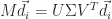
As a linear combination

Another way to see this factorization is as a weighted ordered sum of separable matrices S_i=\vec{u}_i \otimes \vec{v}_i^T each of which has rank(S_i)=1, \forall i:

M = \sum_i \sigma_i \cdot S_i

As an unconstrained optimization

We can also formulate the solution of the svd in terms of an optimization: find the best (minimizes the frobenius norm \|M - B\|_F) approximation B of M that has lower rank \texttt{rank}(B) < \texttt{rank}(M). Dropping an appropriate number of singular values (starting with the smallest) and singular vectors and then reforming a matrix yields the exact global solution. The proof of this lies in the fact that

\| M - B \|_F = \left\| \sum_{i=1}^n \sigma_i \vec{u}_i \vec{v}_i^T - \sum_{i=1}^k \sigma_i \vec{u}_i \vec{v}_i^T \right\|_F = \left\| \sum_{i=k+1}^n \sigma_i \vec{u}_i \vec{v}_i^T \right\|_F = \sqrt{\sigma_{k+1}^2 + \cdots + \sigma_n^2}

This result is the Eckhart-Young theorem.

Condition Number

The condition number of a matrix can be given in terms of its singular values:

k(M) = \|M \| \cdot \| M^{-1} \| = \frac{\sigma_{\max}(M)}{\sigma_{\min}(M)}

A matrix is said to be ill conditioned if the condition number is too large. How large the condition number can be, before the matrix is ill conditioned, is determined by the machine precision.

Tagged with: , ,